Implementing SimCLR using a Callback in fast.ai

Paper Link: (https://arxiv.org/abs/2002.05709)

Overview

In this blog post, we’ll implement SimCLR (A Simple Framework for Contrastive Learning of Visual Representations ) using fastai Callbacks.

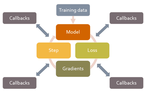
What are Callbacks?

Callbacks are a neat way to inject customizations in your training loop, without having to write the training loop again.

The fast.ai book defines it nicely as:

“A callback is a piece of code that you write, and inject into another piece of code at some predefined point. In fact, callbacks have been used with deep learning training loops for years. The problem is that in previous libraries it was only possible to inject code in a small subset of places where this may have been required, and, more importantly, callbacks were not able to do all the things they needed to do.”

for example: say you want to multiply your training loss by 0.002 before backprop. With callbacks, you can go to the part of your training loop where the loss is calculated (after_loss in fast.ai context) and basically do: loss = 0.002 * loss.

sweet right?

SimCLR summarised

SimCLR was a groundbreaking paper in the field of self-supervised learning in vision by Google.

The idea behind self-supervised learning in vision is : make a model learn better visual representations without human supervision. SimCLR is based on Contrastive learning, where projections of augmented versions of the same image are brought closer (in the latent space) while projections of augmented versions of other images are pushed apart, even if those images are of the same class of object.

The trained model not only does well at identifying different transformations of the same image, but also learns representations of similar concepts (e.g., chairs vs. dogs), which later can be associated with labels through fine-tuning.

SimCLR uses a combination of strong data augmentations, such as random crops, flips, color jitter, and Gaussian blur. These augmentations help the model learn invariant and robust representations by exposing it to diverse variations of the same image.

Pseudocode

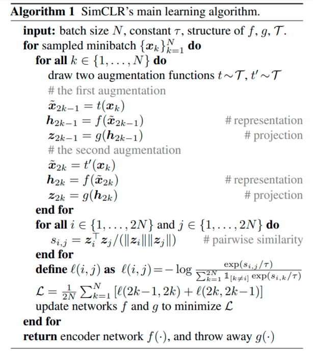
Let’s convert the pseudocode math to python code step-by-step using an example:

# given a batch of two images: (im1, im2)

> we take two different augmentation function V1 and V2 
  and pass the batch through them to obtain two batches 
  corresponding these augmentations:

    (im1_V1, im2_V1) = V1(im1, im2)
    (im1_V2, im2_V2) = V2(im1, im2) 

> encoder 'f' is a resnet50 body and a projection head 
  'g' is a simple MLP. Pass the augmented batches 
  through f and then g. let's call g(f()) = p()

    z1 = p( im1_V1, im2_V1 )
    z2 = p( im1_V2, im2_V2 )

> concatenate the projections z1 and z2:

    z = [projection_im1_v1,
         projection_im2_v1,
         projection_im1_v2,
         projection_im2_v2 ]

> calculate pairwise similarity in z 
  (or the similarity matrix which is nothing 
  but dot product of z with z's transpose)

    sim = z @ z.T

    # similarity pairs look something like this
    sim = im1v1:im1v1  im1v1:im2v1  im1v1:im1v2  imv1:im2v2
          im2v1:im1v1  im2v1:im2v1  im2v1:im1v2  im2v1:im2v2
          im1v2:im1v1  im1v2:im2v1  im1v2:im1v2  imv2:im2v2
          im2v2:im1v1  im2v2:im2v1  im2v2:im1v2  im2v2:im2v2
 
    # positive pairs = different views of the same image
    # negative pairs = everything else in the matrix except diagonal elements

> apply loss function using the sim matrix

Writing the Callback

class SimCLRCallback(Callback):
  def __init__(self, tau=0.1):
    super().__init__()
    self.aug_pipelines = [Pipeline([RandomResizedCrop(224), *aug_transforms(p_lighting=1.0), Normalize.from_stats(*imagenet_stats)]),
                         Pipeline([RandomResizedCrop(224), Normalize.from_stats(*imagenet_stats)])]
    self.info = {}
    self.tau = tau


  def before_batch(self):
    images = self.learn.xb
    self.view_1 = self.aug_pipelines[0](images)
    self.view_2 = self.aug_pipelines[1](images)
    self.learn.xb = self.view_1


  def after_pred(self):
    z1 = self.learn.pred
    z2 = self.learn.model(*self.view_2)
    z = torch.cat([z1, z2], dim=0)
    z = F.normalize(z, dim=1)

    self.sims = z @ z.t() / self.tau
    self.pos = [self.sims[i, i+len(z)//2] for i in range(len(z)//2)]
    self.pos = torch.tensor(self.pos, dtype=self.learn.x.dtype , device=self.learn.x.device)
    self.pos = torch.exp(torch.cat([self.pos]))

    neg_list = []
    for i in range(len(z)//2):
      i_neg = [self.sims[i, j] for j in range(len(z)) if j != i and j != i+len(z)//2]
      neg_list.append(i_neg)

    neg_list = torch.tensor(neg_list, dtype=self.learn.x.dtype , device=self.learn.x.device)
    self.neg = torch.exp(neg_list)
    self.contrastive_loss = -torch.log(self.pos / (self.pos.sum() + self.neg.sum())).mean()  # Contrastive loss


  def after_loss(self):
    self.learn.loss = self.contrastive_loss

Drawbacks of SimCLR

1. SimCLR requires a high batch size.
2. SimCLR requires a large amount of data to learn meaningful representations.

To Do

Plot visualisation of SimCLR learned representations